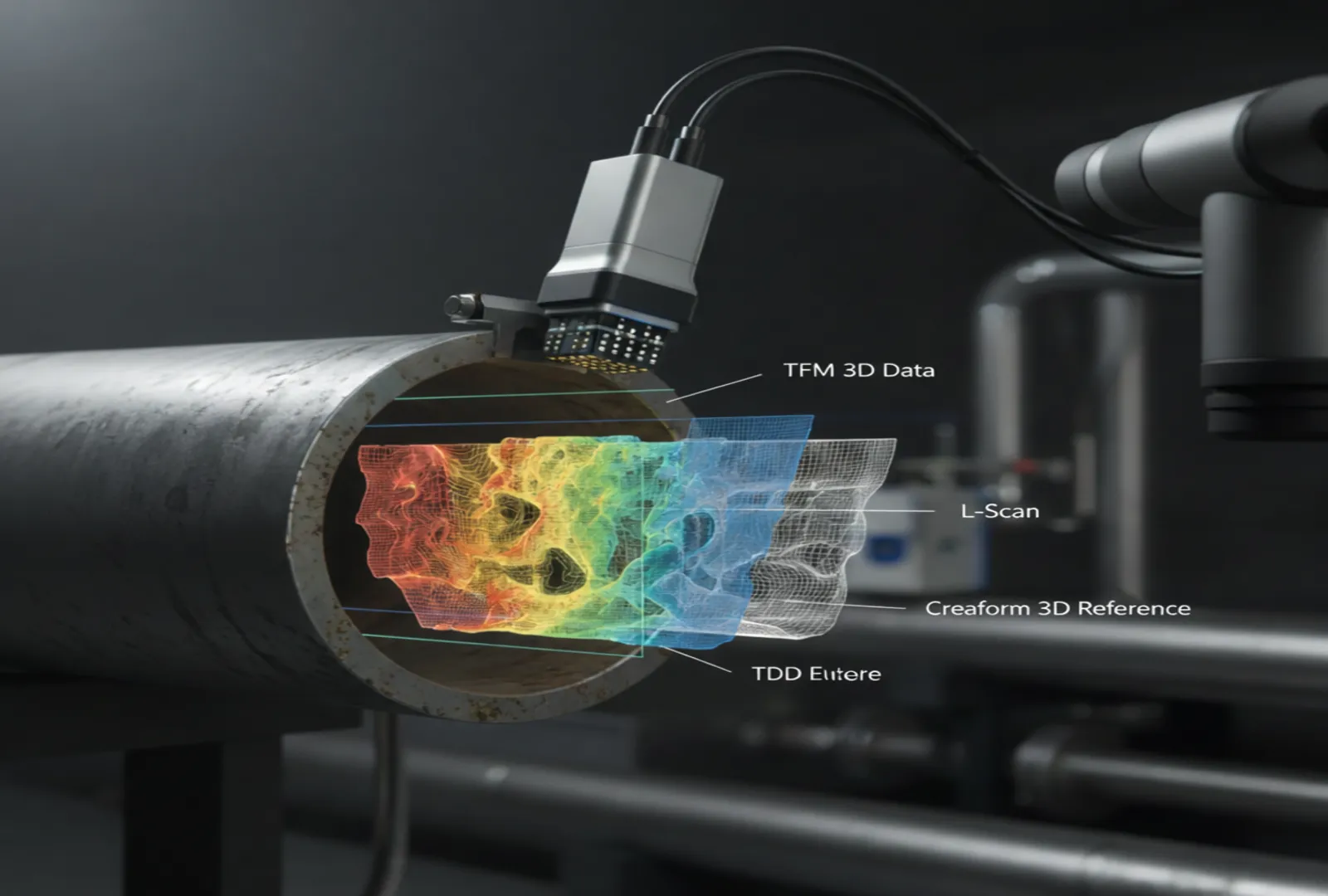
Ultrasound corrosion-mapping techniques have evolved from single-point readings to linear scan mapping and now the Total Focusing Method (TFM). This study evaluates how probe type, scan strategy, and post-processing methods affect the accuracy of corrosion characterization. Two artificially machined corrosion features—precisely 1 mm apart in depth, were scanned using phased-array probes and analyzed through TFM, linear scan (L-scan), and high-accuracy 3D laser mapping. By comparing qualitative and quantitative metrics, the study identifies optimal setups for maximizing accuracy and repeatability in corrosion assessment, a process valuable for industries such as oil & gas and pressure-vessel inspection.
The corrosion mapping purpose
Corrosion reduces pipe and vessel wall thickness in unpredictable ways. Phased-array corrosion mapping visualizes this thickness variation as a color-coded image. An effective corrosion map must be high-resolution and three-dimensional, allowing asset owners to monitor damage progression and determine whether mitigation strategies are working. High-fidelity maps provide insight into corrosion evolution across maintenance cycles.
Asset owners rely on repeated, accurate thickness mapping to avoid premature equipment replacement. With corrosion costing the U.S. economy an estimated $276 billion annually, reliable inspection influences maintenance planning and operational safety.
Modern corrosion-management software incorporates corrosion rate modeling, environmental factors, anomaly detection, and predictive thickness calculations. When combined with ultrasound mapping and 3D surface reconstruction, these tools generate highly accurate digital models for determining safe operating limits and planning repairs.
Comparing L-scan to TFM mapping to a 3D reference
TFM imaging, unlike L-scan,focuses every point in the region of interest, improving defect clarity and depth accuracy. However, TFM and L-scan do not always produce identical corrosion-area measurements. This study compares both ultrasound methods with the “true profile,” obtained from a Creaform 3D scanner, to evaluate accuracy limits and imaging behavior.
Methodology
Two identical machined corrosion patches were digitized using a 3D scanner at 1 mm × 1 mm resolution, matching the ultrasound grid. The scanner’s 0.025 mm precision makes it nearly six times more accurate than a 10 MHz ultrasound probe.
Three 64-element probes—3.5 MHz, 5 MHz, and 10 MHz—were used to capture synchronized TFM and L-scan datasets. Post-processing was performed using UTStudio+ and CIVA tools to extract area, thickness, and profile information.
Results
Depth measurements
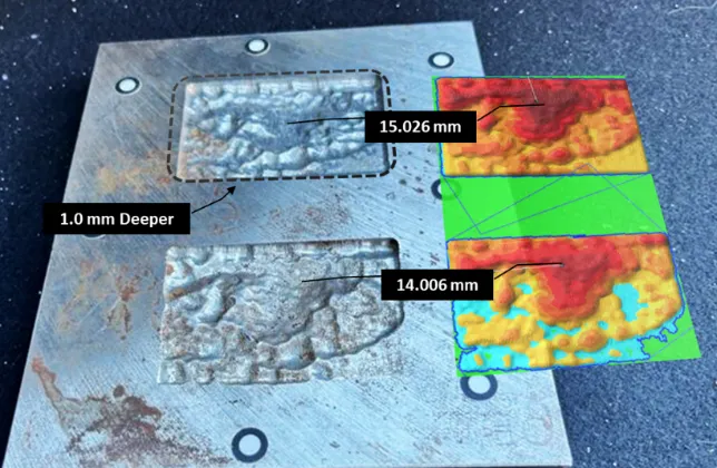
Across all scans and frequencies, both techniques measured minimum thickness within 5% error. TFM demonstrated superior depth precision (±0.025 mm), whereas L-scan was limited by coarser sample spacing (±0.05 mm). Although both methods accurately detected the 1 mm depth change, TFM showed better repeatability for long-term monitoring.
Damaged area evaluation
Defect with beam width: higher frequencies produce narrower beams and smaller mapped areas. Results for the 10 MHz probe are reproduced below, just as in the original format.
Damage #1 table
| Scan Type | Area (mm2) | Relative Difference to Ref. (%) |
| Creaform (Reference) | 2552 | – |
| L-Scan | 2754 | +7.33 |
| TFM | 2348 | -8.69 |
Damage #2 table
| Scan Type | Area (mm2) | Relative Difference to Ref. (%) |
| Creaform (Reference) | 4235 | – |
| L-Scan | 4314 | +1.83 |
| TFM | 4100 | -3.29 |
L-scan consistently defect area due to larger beam width. TFM tends to underestimate area at high frequencies but slightly oversized at 3.5 MHz because the wider beam disperses the echo.
Beam width decreases with frequency, from 6.6 mm at 3.5 MHz to 2.3 mm at 10 MHz, which directly drives mapping differences in both L-scan and TFM. Lower frequencies produce broader echo scattering, although thickness results remain consistent.
Qualitative Comparison
Shape accuracy
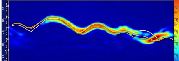
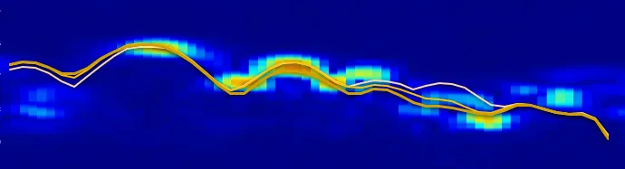
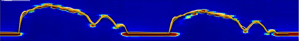
TFM produced profiles that more closely matched the Creaform 3D scan, whereas L-scan captured minimum-thickness points but lacked curved-surface fidelity.
Table 1 – TFM (left) vs L-scan (right) side-view overlay
Profile B-scan in Two-Axis Mapping
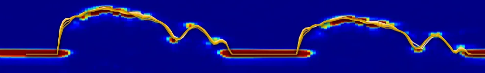
Both TFM and L-scan provide visually consistent B-scan thickness profiles, though TFM cannot focus along the probe’s passive axis.
Table 2 – TFM B-scan (top) and L-scan side view (bottom)
TFM profiler overlaid to 3D laser data
TFM’s high index-axis resolution (0.1 mm) allows extremely accurate profile extraction. When TFM profiler lines were overlaid on Creaform data, they nearly aligned perfectly. Missing TFM pixels have minimal effect on overall profile shape if appropriate thresholds and sampling windows are set.
3D on 3D comparison
A full 3D export of TFM data was not possible, but 2D profiles aligned well with laser scan equivalents. For engineering assessments, API 579 requires thickness, waveform, and geometry inputs—TFM and laser scanning complement each other by providing exterior and interior surface information.
Probe and scan optimization
Frequency and area
The optimal ultrasound frequency for corrosion mapping is 5–7.5 MHz. Higher frequencies benefit thin materials and near-surface resolution but may undersize defect areas.
TFM scan resolution
Resolution can be reduced asymmetrically (0.2 mm index × 0.1 mm depth) while maintaining nearly identical image output, increasing acquisition speed nearly two-fold.
This paper demonstrates that it is possible to decrease the active receive aperture during the FMC step without compromising image quality. The study shows that having 8 to 32 receiving elements per transmitting element is sufficient to maintain image quality. By reducing the active receive aperture, scan speed can be improved by a factor of 2 depending on the record FMC strategies.
Conclusions
Integrating TFM imaging with 3D post-analysis tools yields highly accurate corrosion profiles that closely match physical geometry. TFM’s precision enables reconstruction of corrosion shapes with excellent fidelity. For corrosion mapping, probes in the 5–7.5 MHz range offer the best balance of resolution and accurate area representation. Despite similar thickness measurements between TFM and L-scan, their differing imaging behaviors require careful interpretation. As new imaging techniques evolve, consistency in long-term corrosion monitoring remains an important challenge.
Quantitative area comparisons alone do not describe echo behavior. L-scan and TFM respond differently to pitting, erosion, and small reflectors. Because TFM and L-scan exhibit distinct imaging characteristics, the authors recommend using both methods during a transition period to maintain classification consistency.
This article was developed by specialists from Sonatest and published as part of the seventh edition of Inspenet Brief February 2026, dedicated to technical content in the energy and industrial sector.